Introduction
Breast Cancer (BC), following skin cancer, is the most commonly diagnosed cancer in women [ 1 ]. After lung cancer, which has the highest mortality rate, BC has the second-highest incidence among all cancer types [ 2 ]. The International Agency for Research on Cancer, a part of the World Health Organization, projects that by 2030, BC cases will rise to 27 million new diagnoses [ 3 ]. A pathologist’s diagnosis of BC is determined by analyzing histological sample images under a microscope. The problem with this type of diagnosis is the variability in opinions among different individuals and the significance of their experience level. In a research study, the diagnoses of pathologists matched in only 75% of the cases [ 4 ]. Recent advancements in digital image processing and machine learning have led to the design of computer-aided diagnosis systems that assist pathologists in being more productive, objective, and consistent in diagnosis [ 5 ].
Automated image processing for cancer diagnosis has been the subject of many studies for over 40 years. These studies employ a range of techniques from the analysis of cancer cell nuclei features using specialized image processing software and computerized nuclear morphometry [ 6 - 7 ] to employing deep learning [ 8 - 13 ]. Current research indicates that Convolutional Neural Networks (CNNs) outperform traditional hand-crafted feature extraction techniques in both speed and reliability for BC classification tasks [ 8 , 14 - 15 ]. However, the limited data available in medical imaging often makes it impractical to train networks effectively from scratch. Therefore, utilizing pre-trained networks for feature extraction offers a viable solution to this challenge [ 16 ]. This approach utilizes pre-trained CNNs to extract deep features, which are then fed into a classifier to make the final decision. Still, extracting distinct and useful features, which is highly important, is challenging. To address this issue, researchers focus on either feature extraction from multiple layers or exploring distinctive features through attention mechanisms.
A study by Spanhol et al. evaluated deep features from the pre-trained AlexNet using the BreakHis dataset for BC classification [ 8 ]. Initially, the performance of deep features from the fully connected layers six, seven, and eight using a logistic regression classifier was assessed separately. In addition, an evaluation was conducted by combining the features mentioned above. Combining features from different fully connected layers led to a 0.3% improvement in classification accuracy, resulting in an accuracy of 86.3% at 200× magnification. A study by Gupta et al. utilized the DenseNet and the BreakHis dataset [ 9 ]. This research evaluated the impact of extracting features from different layers (low-mid-high) on the performance. The approach involved extracting features based on the layer’s order and selecting the top-ranking features (<3000) for each layer using the Extreme Gradient Boosting (XGBoost) score. The study shows that the lower layers significantly impact classification performance at 40× magnification, achieving an accuracy of 94.7%. In contrast, an analysis that considers only the higher layers yields an accuracy of approximately 92%. Additionally, the higher layers play a more critical role, due to the more detailed information, at higher magnifications (400×). At intermediate magnifications (100× and 200×), the contribution of all layers is similar. In another study, Gupta et al. focused on classifying BC histopathology images from the BreakHis dataset using multi-layered features from the pre-trained ResNet [ 10 ]. The process involved first extracting features from the ith layer and then reducing their dimensionality using the XGBoost algorithm. These reduced features were fed into Support Vector Machine (SVM) classifier. An information-theoretic measure was utilized to identify an optimal set of layers. Mutual Information (MI) between the predicted and true labels was evaluated to select a subset of layers for feature extraction. The study investigated the multi-layered model in two ways: by evaluating multi-layered features individually and by analyzing a multi-layered model that integrates multi-layered features. The findings show that considering feature integration enhances performance. This approach achieved an accuracy of 96.81% at 40× magnification.
Zou et al. employed attention mechanisms and high-order statistical representations within residual networks to identify distinctive features in the classification of histopathology images from the BreakHis and ICIAR/BACH datasets [ 11 ]. This research improved classification performance, achieving 99.29% accuracy at patient-wise on the BreakHis dataset for the 40× magnification, and 85% on the ICIAR/BACH dataset. By capturing more discriminant features, Ashurov et al. also improved the malignancy detection in BC histopathology images, focusing on feature extraction from pre-trained networks with attention mechanisms on the BreakHis dataset [ 12 ]. The study used Xception, VGG19, ResNet50, MobileNet, and DenseNet121, all enhanced with the Convolutional Block Attention Module (CBAM). Features extracted from these networks were fed into a softmax classifier. The Xception network achieved classification accuracy between 99.2% and 99.5%. Using an attention-based deep network in VGG16, Roy et al. focuses on classifying histopathology images at 40× magnification in the BreakHis dataset [ 13 ]. The study addresses both binary classification between benign and malignant classes and the classification of subtypes within each class. The proposed method increased the binary classification accuracy from 89.3% to 90.4%, and by addressing the class imbalance issue, this accuracy further improved to 97.7%. In the classification of benign subtypes, the method achieved an accuracy ranging from 77.1% to 88.5%, and in the classification of malignant subtypes, accuracy ranged from 77.2% to 98.3%. Azmoodeh-kalati et al. [ 17 ] utilized EfficientNetV1 and EfficientNetV2 architectures for the binary classification of the BreakHis dataset. To overcome the limitation of annotated data, they applied data augmentation and transfer learning techniques. Model interpretability was enhanced using the Gradient-weighted Class Activation Mapping (Grad-CAM) method to highlight discriminative regions relevant to the classification decision. Moreover, ensemble learning strategies specifically unweighted averaging and majority voting were employed to combine predictions from multiple trained models. The framework achieved a classification accuracy of 99.58% on the dataset.
Contrary to the common assumption that features extracted from the last layer of a network yield the best classification performance, research has shown that relying solely on features from this layer can adversely affect performance. Therefore, the last layer cannot extract all distinctive features and often produces similar, less discriminative ones. Thus, it is essential to consider distinct features from other layers. In this research, we propose a layer selection method to identify and utilize the most relevant features from a set of effective layers, aiming to improve performance in malignancy diagnosis in histopathology images. MI between each layer’s features and true labels innovatively is employ to select the most informative features. The proposed method is evaluated on three different CNN architectures.
Material and Methods
In this analytical computational study, two publicly available datasets were used to evaluate the proposed method. The BreakHis dataset consists of 7,909 clinically representative microscopic images of breast tumor tissues categorized as benign or malignant, collected from 82 patients (24 benign tumors and 58 malignant tumors) using various magnification levels: 40×, 100×, 200×, and 400× [ 18 ]. This dataset was developed in collaboration with the P&D Laboratory– Pathological Anatomy and Cytopathology, Parana, Brazil. four histologically distinct types of benign breast tumors are included in the dataset: Adenosis (A), Fibroadenoma (F), Phyllodes Tumor (PT), and Tubular Adenoma (TA); as well as four types of malignant breast tumors: Ductal Carcinoma (DC), Lobular Carcinoma (LC), Mucinous Carcinoma (MC), and Papillary Carcinoma (PC). The number of images for each tumor type at each magnification is mentioned in Table 1. All samples were obtained via Surgical Open Biopsy (SOB) and stained using Hematoxylin and Eosin (H&E) methods. Each image filename encodes detailed metadata, including the biopsy procedure method, magnification factor, cancer type and subtypes, and patient identification. The second dataset, ICIAR/BACH, is comprising 400 H&E-stained histopathology images of BC [ 19 ]. It is categorized into four groups: normal, benign, in situ carcinoma, and invasive carcinoma, with each group containing 100 breast microscopic images. Details about the number of patients in this dataset are not provided. Sample images at each magnification for both malignant and benign categories from the BreakHis dataset and sample images from the ICIAR/BACH dataset across all four classes, are shown in Figure 1.
| Magnification | Benign | Malignant | Total | ||||||
|---|---|---|---|---|---|---|---|---|---|
| A | F | TA | PT | DC | LC | MC | PC | ||
| 40× | 114 | 253 | 109 | 149 | 865 | 156 | 205 | 145 | 1996 |
| 100× | 113 | 260 | 121 | 150 | 903 | 170 | 222 | 142 | 2081 |
| 200× | 111 | 264 | 108 | 140 | 896 | 163 | 196 | 135 | 2013 |
| 400× | 106 | 237 | 115 | 130 | 788 | 137 | 169 | 138 | 1820 |
| Number of patients | 4 | 10 | 3 | 7 | 38 | 5 | 9 | 6 | 82 |
| A: Adenosis, F: Fibroadenoma, TA: Tubular Adenoma, PT: Phyllodes Tumor, DC: Ductal Carcinoma, LC: Lobular Carcinoma, MC: Mucinous Carcinoma, PC: Papillary Carcinoma | |||||||||
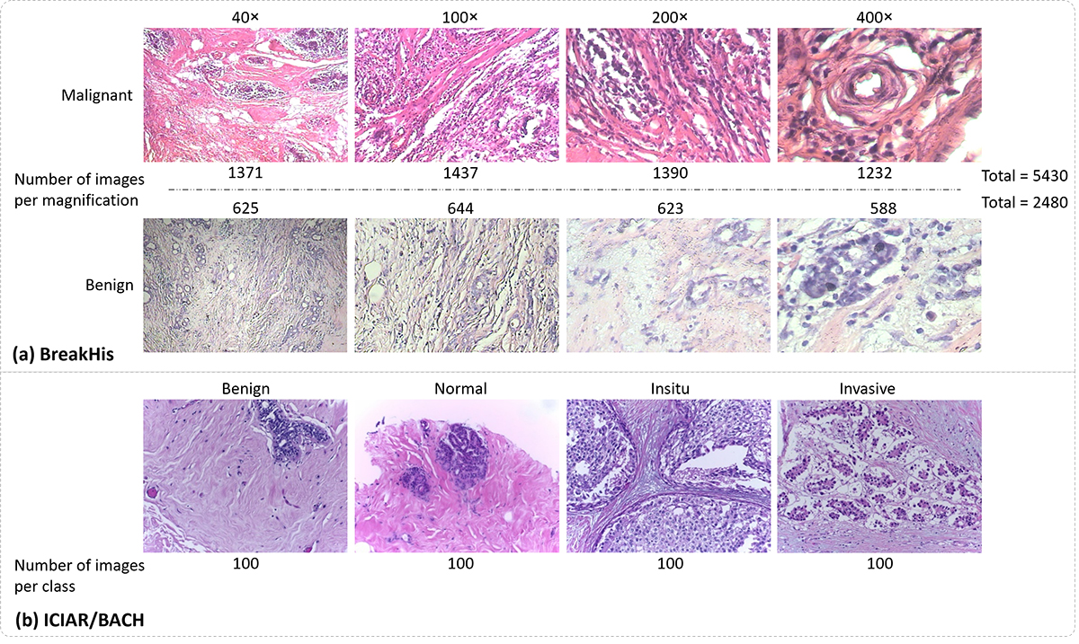
Figure 1. (a) Sample images from the BreakHis dataset in two classes, benign and malignant, at four different magnifications (the number of images per magnification is included), and (b) sample images from the ICIAR/BACH dataset in four different classes (the number of images per class is included).
Method
This research proposes a method to select effective layers and concatenate the distinctive and significant deep features extracted from these layers in each network to achieve a better performance in classifying tumorous and healthy tissues. In this study, deep features from different layers were extracted from the pre-trained VGG19, DenseNet, and ConvNextTiny networks operating in transfer learning mode. Features from the initial layers have been disregarded due to the low-level general content and the high dimensionality of their feature vectors. Therefore, features from the higher layers that provide more important information from the data were extracted. These layers capture high-level features of complex patterns such as shape, texture, and objects [ 20 ], which are very useful in classification tasks. Additionally, these layers have fewer neurons compared to the initial layers, resulting in feature vectors with smaller sizes, leading to memory savings and faster processing [ 21 ].
To measure the effectiveness of the features extracted from each layer, MI between each layer’s features and the set of true labels was computed, and a set of layers based on the maximum MI was selected. To address the challenges posed by the high dimensions of the feature vector (relative to the number of data), the Principal Component Analysis (PCA) algorithm, considering a full range of Cumulative Explained Variance (CEV) from 5% to 100%, to determine the optimal number of Principal Components (PCs) [ 22 ], has been applied to the feature vector of the selected layers. To select the optimal CEV, we evaluated 10 random data splits and used boxplots analysis, mean accuracy, and result stability to identify the best value.
Finally, the transformed features from the selected layers in each network were concatenated to generate a comprehensive feature set for the respective network and fed into an SVM classifier as input. A summary of the proposed method is illustrated in Figure 2.
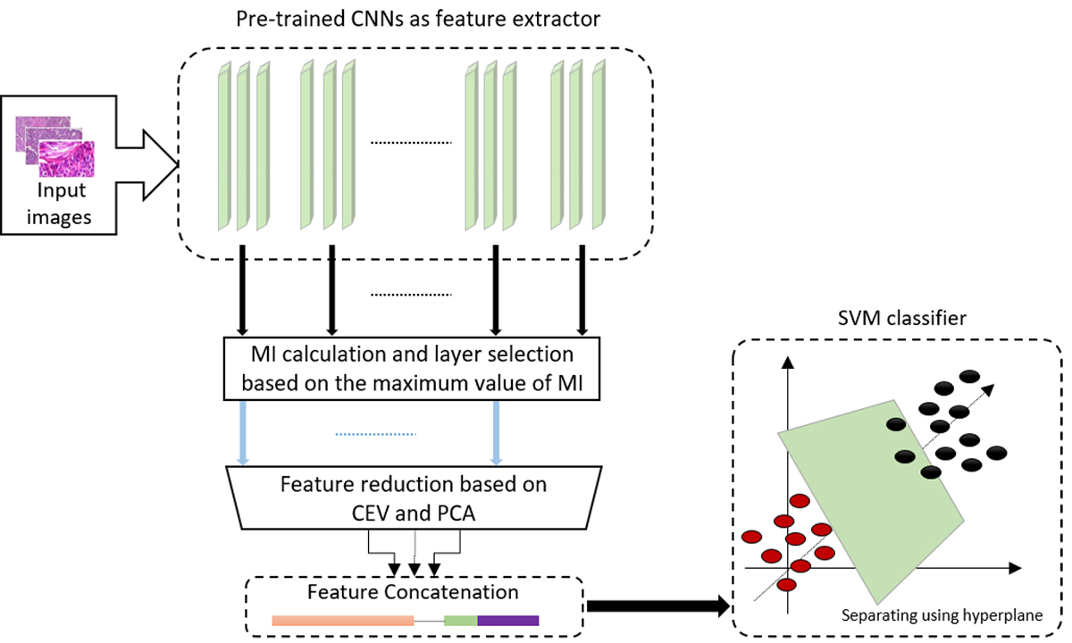
Figure 2. The diagram of the proposed method(Convolutional Neural Networks (CNNs), Mutual Information (MI), Cumulative Explained Variance (CEV), Principal Component Analysis (PCA), Support Vector Machine (SVM)).
Investigated layers of networks
Initial layers typically capture low-level features, such as corners and edges. As the depth of the architecture increases, the network starts to learn more complex, high-level features, which are highly advantageous for classification tasks. Additionally, due to the reduction in the number of neurons in the upper layers, feature extraction leads to memory savings and an increase in processing speed [ 20 ]. As a result, feature extraction from the lower layers was excluded, and the focus was placed on extracting features from the higher layers of the network. The blocks investigated for feature extraction are shown in blue in Figure 3 for each network. In addition, features also were extracted from the final layer before the classifier in each network referred to as the baseline in this study for comparison purposes.
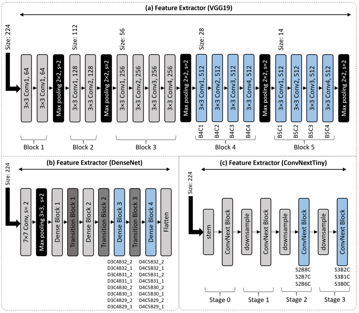
Figure 3. Investigated layers in the (a) VGG19, (b) DenseNet, and (c) ConvNextTiny networks. The blocks used for feature extraction are highlighted in blue, and the names of the layers in each block are indicated.
VGG19: This network was introduced by researchers at the University of Oxford to participate in the ImageNet image classification challenge [ 23 ]. The VGG19 network consists of 19 layers, including 16 convolutional layers and 3 fully connected layers. The pre-trained weights of this network, based on the ImageNet dataset, are useful for feature extraction from other images or for fine-tuning. In the VGG19 network, feature extraction focused on the blocks 4 and 5 as shown in blue color in Figure 3a. The feature vector dimensions for these blocks are 401,408 and 100,352, respectively, while the baseline has a dimension of 25,088.
DenseNet: DenseNet was introduced by Huang et al. [ 24 ]. The main innovation of the DenseNet architecture lies in its dense connections, where each layer receives inputs from all the preceding layers. As a result, the ith layer receives the feature maps of all the previous layers as its input. In this network, feature extraction is performed from blocks 3 and 4 (Figure 3b), which produce feature vectors with dimensions of 1,568, 6,272, and 25,088. Each of these blocks contains 32 convolutional layers. Among these, features were extracted from blocks 29 to 32, each containing two convolutional layers. The baseline layer in this network has a dimension of 81,536.
ConvNextTiny: This network, inspired by the design of Vision Transformers (ViT), was introduced by Liu et al. [ 25 ]. In their research, Liu and his team redesigned standard convolutional neural networks, drawing inspiration from ViT and uncovering key insights that led to improved performance. The outcome of this research was the introduction of a new group of convolutional models called ConvNext. Built on earlier convolutional networks, ConvNext models performed better than ViT in classifying ImageNet data. In the ConvNextTiny network, feature extraction was performed from stages 2 and 3 (Figure 3c). Each stage contains convolutional layers. In stage 3, features were extracted from all three 2D convolutional layers, which have dimensions of 37,632. In stage 2, feature extraction was carried out from the top three 2D convolutional layers, which have an output dimension of 75,264, while the baseline has a dimension of 37,632.
Layer selection based on mutual information
The MI is a measure used to determine how much information about one random variable can be obtained from another. MI is particularly suitable for assessing the relevance between two datasets for several reasons: it identifies any relationship between the datasets, is not sensitive to the size of the datasets, and it provides a straightforward way to describe the amount of shared information. Since MI is based on information theory, it has a solid theoretical foundation [ 26 ]. Therefore, the MI was used to assess the effectiveness of features extracted from each layer and to select the effective layers. MI was computed between each layer’s features and true labels. By plotting the MI histogram for different layers and networks, MI across different layers from various networks exhibited a similar distribution. Figure 4 shows the MI distribution calculated for a 100× magnification of the layer B4C4 in the VGG19 network, the layer D3B32_2 in the DenseNet, and the layer S3B2C in the ConvNextTiny network. This distribution closely resembles the well-known Rayleigh distribution. As a result, further investigation was conducted on the Rayleigh distribution, and key parameters for each MI set, including maximum, minimum, mean, standard deviation, mode, and median values, were calculated. Finally, the maximum MI value was selected as the criterion for layer selection since a higher MI signifies more information about the other variable.
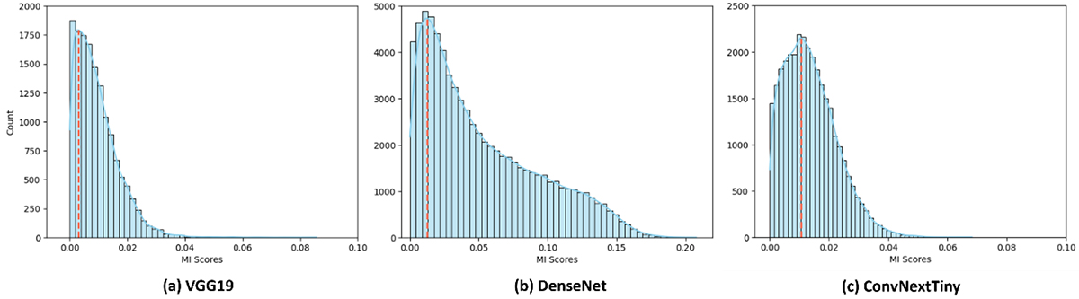
Figure 4. Histogram of Mutual Information (MI) scores for 100× magnification: (a) B4C4 layer in VGG19, (b) D3B32_2 layer in DenseNet, and (c) S3B2C layer in ConvNextTiny, where the red dashed line indicates the mode.
Feature reduction
Extracting deep features from pre-trained models results in high-dimensional feature vectors, which are typically not fed directly into the classification algorithm due to the risk of overfitting [ 27 ]. Therefore, after selecting the effective layers, it is necessary to apply a method for dimensionality reduction of the feature vectors from selected layers. The PCA algorithm is a feature extraction method that generates a new feature vector by linearly combining the original features. In other words, by applying a linear transformation to the original features, a new set of features is created that preserves a specified amount of variance in the data [ 28 ]. By applying PCA to the feature vectors of effective layers and determining the optimal number of components through changes in CEV [ 22 ], the issue of overfitting is alleviated, and the computational load during the classification stage is reduced.
Classifier
The SVM algorithm is a supervised learning algorithm in machine learning. This algorithm is widely used in classification and regression problems. In the field of data classification, the primary goal of SVM is to find the best hyperplane to correctly separate the data from one another. In cases where the data is not linearly separable, SVM addresses this issue by the kernel trick [ 29 ], where it applies functions to transform the input space from lower to higher dimensions. To utilize the SVM algorithm for classification, it is necessary to select an appropriate kernel and optimally tune several parameters. For this purpose, grid search cross-validation was employed to identify the optimal kernel and parameter settings. Among the various kernels, such as Radial Basis Function (RBF), linear, polynomial, and sigmoid, the RBF kernel demonstrated superior performance. Accordingly, the penalty parameter C was set to 5, and the gamma parameter was also adjusted dynamically based on the number of features and the variance of the data. The dataset was divided into a training set (80%) and a test set (20%) using the split method in image-wise investigation. The results were reported as the average across 10 random splits.
Evaluation
To investigate the performance of the proposed method using the BreakHis dataset, the model’s performance was evaluated both image-wise and patient-wise for each magnification separately. In the ICIAR/BACH dataset, the model’s performance was evaluated only image-wise (due to the lack of information regarding the patient’s ID). In the image-wise evaluation, the focus was on the number of correctly classified images in the studied datasets. In this study, the metrics of accuracy, precision, recall, and F1-score were examined. These metrics were computed by True Positive (TP), True Negative (TN), False Positive (FP), and False Negative (FN). In medical diagnosis, the model needed to perform well on each patient’s data, and the results were also reported for each patient separately. In the patient-wise evaluation, the average of correctly classified images per patient was important. If NP is the total number of patients, is the total number of correctly classified images for patient P, and is the total number of images for patient P, then the classification accuracy of patient-wise is computed as follows:
Results
The maximum value of MI of the investigated layers in the VGG19 network using the BreakHis and ICIAR/BACH datasets was reported in Table 2. The selected layers were highlighted in bold. Layers marked with “—” were excluded from further evaluation. For the BreakHis dataset, three layers were chosen to ensure an adequate feature set for classification after dimensionality reduction, while keeping the model complexity manageable. For the ICIAR/BACH dataset, four layers were selected to provide sufficient features to distinguish among the four different classes. Furthermore, Table 2 presented the image-wise classification accuracy utilizing the features from the selected layers, both before and after the implementation of PCA. It also included the optimal number of components and their corresponding CEV.
| Dataset | Mag. | Metrics | Layers | |||||||
|---|---|---|---|---|---|---|---|---|---|---|
| Block 5 Feature vector size = 100352 | Block 4Feature vector size = 401405 | |||||||||
| B5C4 | B5C3 | B5C2 | B5C1 | B4C4 | B4C3 | B4C2 | B4C1 | |||
| BreakHis | 40× | MImax | 0.0801 | 0.0955 | 0.0822 | 0.1055 | 0.1002 | 0.0973 | 0.1367 | 0.1256 |
| Accuracy | - | - | - | 90.62±1.12 | - | - | 90.07±1.68 | 90.94±1.11 | ||
| CEV, #cmp | - | - | - | 20, 77 | - | - | 15, 26 | 20, 24 | ||
| Accuracy w/PCA | - | - | - | 90.77±1.37 | - | - | 92.82±1.00 | 94.05±0.8 | ||
| 100× | MImax | 0.0749 | 0.0857 | 0.1048 | 0.1044 | 0.1224 | 0.1244 | 0.1656 | 0.1437 | |
| Accuracy | - | - | - | - | - | 87.89±1.46 | 89.64±1.11 | 90.95±1.40 | ||
| CEV, #cmp | - | - | - | - | - | 10, 32 | 15, 32 | 20, 36 | ||
| Accuracy w/PCA | - | - | - | - | - | 92.55±0.9 | 94.01±1.42 | 93.61±1.12 | ||
| 200× | MImax | 0.1108 | 0.1249 | 0.1178 | 0.1466 | 0.1376 | 0.1514 | 0.1724 | 0.1774 | |
| Accuracy | - | - | - | - | - | 88.26±1.56 | 90.74±1.06 | 90.84±1.13 | ||
| CEV, #cmp | - | - | - | - | - | 10, 34 | 15, 35 | 20, 36 | ||
| Accuracy w/PCA | - | - | - | - | - | 92.38±0.7 | 94.06±1.24 | 94.39±1.04 | ||
| 400× | MImax | 0.1053 | 0.0988 | 0.0940 | 0.1168 | 0.1180 | 0.1349 | 0.1497 | 0.1421 | |
| Accuracy | - | - | - | - | - | 86.40±2.03 | 86.97±1.90 | 86.75±2.23 | ||
| CEV, #cmp | - | - | - | - | - | 5, 8 | 10, 14 | 15, 19 | ||
| Accuracy w/PCA | - | - | - | - | - | 88.81±1.18 | 91.64±1.04 | 91.84±1.15 | ||
| ICIAR/BACH | - | MImax | 0.1817 | 0.2028 | 0.1988 | 0.1650 | 0.1800 | 0.1848 | 0.2174 | 0.2160 |
| Accuracy | - | 68.12±3.45 | 66.24±4.67 | - | - | - | 61.50±6.36 | 60.12±6.67 | ||
| CEV, #cmp | - | 25, 30 | 60, 128 | - | - | - | 30, 48 | 20, 17 | ||
| Accuracy w/PCA | - | 66.50±4.19 | 64.87±4.94 | - | - | - | 62.87±7.09 | 63.12±5.3 | ||
| Mag.: Magnification, MI: Mutual Information, CEV: Cumulative Explained Variance, #cmp: number of components | ||||||||||
The results indicated that applying the PCA with consideration of a specific level of CEV effectively reduced the feature vector size from 100,352 in block 5 and from 401,405 in block 4 to a value below 100. This reduction enhanced classification accuracy within the BreakHis dataset, although a slight decrease in classification accuracy of some layers within the ICIAR/BACH dataset was observed. The selected layers for the BreakHis dataset at 40× magnification included layers B5C1, B4C2, and B4C1. At 100×, 200×, and 400× magnifications, the selected layers were B4C3, B4C2, and B4C1. The selected layers for the ICIAR/BACH dataset were B5C3, B5C2, B4C2, and B4C1.
Table 3 reported the maximum MI values of the investigated layers of the DenseNet using the BreakHis and ICIAR/BACH datasets. The selected layers were indicated in bold. Layers marked with “—” were excluded from further evaluation. Due to the smaller size of the feature vector in this network, a greater number of layers could be analyzed. As a result, three layers from each block under investigation were selected for both datasets, ensuring representation from various stages of the network. Additionally, Table 3 displayed the image-wise classification accuracy obtained from these layers before and after the implementation of PCA. It also outlined the optimal number of components and their corresponding CEV.
| Dataset | Mag. | Metrics | Layers | Dense Block 4 | |||||||
|---|---|---|---|---|---|---|---|---|---|---|---|
| D4C5B32_2 FVS =1568 | D4C5B32_1 FVS =6272 | D4C5B31_2 FVS =1568 | D4C5B31_1 FVS =6272 | D4C5B30_2 FVS =1568 | D4C5B30_1 FVS =6272 | D4C5B29_2 FVS =1568 | D4C5B29_1 FVS =6272 | ||||
| BreakHis | 40× | MImax | 0.1879 | 0.1973 | 0.1879 | 0.1698 | 0.1694 | 0.1905 | 0.1826 | 0.1851 | |
| Accuracy | 85.47±1.94 | 85.02±1.59 | - | - | - | 85.02±1.77 | - | - | |||
| CEV, #cmp | 100, 1568 | 100, 1568 | - | - | - | 100, 1568 | - | - | |||
| Accuracy w/PCA | 87.37±2.04 | 88.00±2.18 | - | - | - | 87.70±1.52 | - | - | |||
| 100× | MImax | 0.1763 | 0.1867 | 0.1763 | 0.1876 | 0.1620 | 0.1849 | 0.1958 | 0.1839 | ||
| Accuracy | - | 83.49±1.57 | - | 83.42±1.24 | - | - | 81.82±1.29 | - | |||
| CEV, #cmp | - | 100, 2045 | - | 100, 2043 | - | - | 100, 1568 | - | |||
| Accuracy w/PCA | - | 89.19±0.9 | - | 86.95±1.07 | - | - | 84.34±0.9 | - | |||
| 200× | MImax | 0.2228 | 0.2468 | 0.2228 | 0.2464 | 0.2434 | 0.2388 | 0.2122 | 0.2426 | ||
| Accuracy | - | 87.22±1.43 | - | 87.22±1.55 | 89.80±1.89 | - | - | - | |||
| CEV, #cmp | - | 100, 1979 | - | 100, 1568 | 100, 1568 | - | - | - | |||
| Accuracy w/PCA | - | 90.27±1.41 | - | 89.57±1.42 | 89.72±1.85 | - | - | - | |||
| 400× | MImax | 0.1996 | 0.2103 | 0.1996 | 0.1996 | 0.2038 | 0.2083 | 0.1796 | 0.2091 | ||
| Accuracy | - | 84.58±2.51 | - | - | 85.85±1.81 | 85.13±2.50 | - | - | |||
| CEV, #cmp | - | 100, 1791 | - | - | 90, 66 | 90, 570 | - | - | |||
| Accuracy w/PCA | - | 86.92±2.49 | - | - | 87.91±1.68 | 87.92±1.43 | - | - | |||
| ICIAR/BACH | - | MImax | 0.1682 | 0.1895 | 0.1876 | 0.2549 | 0.1618 | 0.1932 | 0.1952 | 0.1949 | |
| Accuracy | - | - | - | 59.25±4.9 | - | - | 48.00±5.09 | 56.37±4.59 | |||
| CEV, #cmp | - | - | - | 100, 398 | - | - | 90, 62 | 100, 398 | |||
| Accuracy w/PCA | - | - | - | 62.25±3.81 | - | - | 48.87±5.25 | 61.62±3.95 | |||
| Dataset | Mag. | Metrics | Layers | Dense Block 3 | |||||||
| D3C4B32_2 FVS = 6272 | D3C4B32_1 FVS = 25088 | D3C4B31_2 FVS = 6272 | D3C4B31_1 FVS = 25088 | D3C4B30_2 FVS = 6272 | D3C4B30_1 FVS = 25088 | D3C4B29_2 FVS = 6272 | D3C4B29_1 FVS = 25088 | ||||
| BreakHis | 40× | MImax | 0.1471 | 0.1618 | 0.1524 | 0.1723 | 0.1763 | 0.1724 | 0.1606 | 0.1506 | |
| Accuracy | - | - | - | 89.12±1.60 | 87.57±1.63 | 87.89±1.82 | - | - | |||
| CEV, #cmp | - | - | - | 95, 71 | 95, 71 | 100, 1568 | - | - | |||
| Accuracy w/PCA | - | - | - | 90.50±1.50 | 89.22±1.27 | 90.15±1.85 | - | - | |||
| 100× | MImax | 0.1478 | 0.1601 | 0.1516 | 0.1745 | 0.1706 | 0.1752 | 0.1479 | 0.1519 | ||
| Accuracy | - | - | - | 88.51±1.22 | 85.08±1.38 | 88.72±1.37 | - | - | |||
| CEV, #cmp | - | - | - | 90, 576 | 100, 2112 | 95, 917 | - | - | |||
| Accuracy w/PCA | - | - | - | 89.92±1.40 | 88.29±1.66 | 90.40±1.17 | - | - | |||
| 200× | MImax | 0.1982 | 0.2038 | 0.2037 | 0.1941 | 0.2126 | 0.2152 | 0.1894 | 0.2023 | ||
| Accuracy | - | 89.87±1.0 | - | - | 88.63±1.26 | 89.25±1.09 | - | - | |||
| CEV, #cmp | - | 95, 916 | - | - | 95, 334 | 80, 195 | - | - | |||
| Accuracy w/PCA | - | 91.34±0.8 | - | - | 89.60±1.52 | 91.31±0.8 | - | - | |||
| 400× | MImax | 0.1901 | 0.1875 | 0.1841 | 0.1809 | 0.1856 | 0.1845 | 0.1829 | 0.1808 | ||
| Accuracy | 85.82±2.31 | 87.22±1.98 | - | - | 85.79±1.78 | - | - | - | |||
| CEV, #cmp | 80, 39 | 80, 184 | - | - | 100, 1791 | - | - | - | |||
| Accuracy w/PCA | 86.20±2.36 | 88.68±1.69 | - | - | 87.25±2.30 | - | - | - | |||
| ICIAR/BACH | - | MImax | 0.1918 | 0.1976 | 0.2423 | 0.2015 | 0.1918 | 0.2373 | 0.1655 | 0.2257 | |
| Accuracy | - | - | 59.25±4.81 | - | - | 61.50±3.94 | - | 57.25±1.99 | |||
| CEV, #cmp | - | - | 95, 191 | - | - | 60, 53 | - | 70, 88 | |||
| Accuracy w/PCA | - | - | 61.25±7.21 | - | - | 61.75±5.89 | - | 57.75±4.36 | |||
| Mag.: Magnification, MI: Mutual Information, CEV: Cumulative Explained Variance, #cmp: number of components | |||||||||||
The results indicated that the implementation of PCA considering a specific amount of CEV reduced the feature vector size and improved classification accuracy simultaneously, although the improvement for the ICIAR/BACH dataset were relatively small. The selected layers for the BreakHis dataset at 40× magnification included layers D3C4B31_1, D3C4B30_2, D3C4B30_1, D4C5B32_2, D4C5B32_1, and D4C5B30_1. At 100× magnification, the selected layers were D3C4B31_1, D3C4B30_2, D3C4B30_1, D4C5B32_1, D4C5B31_1, and D4C5B29_2. At 200× magnification, the selected layers were D3C4B32_1, D3C4B30_2, D3C4B30_1, D4C5B32_1, D4C5B31_1, and D4C5B30_2. At 400× magnification, the selected layers were D3C4B32_2, D3C4B32_1, D3C4B30_2, D4C5B32_1, D4C5B30_2, and D4C5B30_1. The selected layers for the ICIAR/BACH dataset included layers D3C4B31_2, D3C4B30_1, D3C4B29_1, D4C5B31_1, D4C5B29_2, and D4C5B29_1.
Table 4 reported the maximum MI values of the investigated layers in the ConvNextTiny network using the BreakHis and ICIAR/BACH datasets. The layers selected for further analysis were highlighted in bold. Layers marked with “—” were excluded from further evaluation. In this network, a total of six layers were investigated, and three layers were selected for each dataset to contribute to the classification process. This approach preserved the diversity of features while maintaining computational efficiency and avoiding unnecessary complexity. Moreover, Table 4 presented the image-wise classification accuracy utilizing the features from these layers before and after the implementation of PCA. It also included the optimal number of components and their corresponding CEV.
| Dataset | Mag. | Metrics | Layers | |||||
|---|---|---|---|---|---|---|---|---|
| Stage 3 Feature vector size =37632 | Stage 2 Feature vector size =75264 | |||||||
| S3B2C | S3B1C | S3B0C | S2B8C | S2B7C | S2B6C | |||
| BreakHis | 40× | MImax | 0.0660 | 0.0685 | 0.0772 | 0.0689 | 0.0923 | 0.0880 |
| Accuracy | - | - | 93.52±0.7 | - | 94.69±0.8 | 94.53±1.04 | ||
| CEV, #cmp | - | - | 35, 74 | - | 25, 49 | 25, 38 | ||
| Accuracy w/PCA | - | - | 95.35±0.9 | - | 96.67±0.8 | 98.10±0.5 | ||
| 100× | MImax | 0.0870 | 0.0832 | 0.0823 | 0.0789 | 0.1236 | 0.1083 | |
| Accuracy | 91.77±1.98 | - | - | - | 94.20±1.23 | 94.37±1.25 | ||
| CEV, #cmp | 55, 178 | - | - | - | 25, 49 | 30, 62 | ||
| Accuracy w/PCA | 94.01±1.35 | - | - | - | 96.26±0.8 | 96.28±1.08 | ||
| 200× | MImax | 0.0779 | 0.0853 | 0.0777 | 0.0907 | 0.1198 | 0.1319 | |
| Accuracy | - | - | - | 90.59±1.46 | 93.27±1.06 | 93.89±1.06 | ||
| CEV, #cmp | - | - | - | 15, 36 | 25, 54 | 30, 66 | ||
| Accuracy w/PCA | - | - | - | 94.09±1.31 | 96.00±0.9 | 97.07±0.7 | ||
| 400× | MImax | 0.0535 | 0.0579 | 0.0645 | 0.0675 | 0.0890 | 0.1244 | |
| Accuracy | - | - | - | 88.46±1.68 | 91.40±1.72 | 91.26±1.38 | ||
| CEV, #cmp | - | - | - | 20, 70 | 25, 58 | 20, 26 | ||
| Accuracy w/PCA | - | - | - | 91.34±2 | 95.08±0.7 | 95.10±0.95 | ||
| ICIAR/BACH | - | MImax | 0.2363 | 0.2528 | 0.2437 | 0.2690 | 0.2245 | 0.2007 |
| Accuracy | - | 79.12±4.22 | 86.49±3.20 | 75.37±3.44 | - | - | ||
| CEV, #cmp | - | 45, 52 | 30, 26 | 20, 26 | - | - | ||
| Accuracy w/PCA | - | 78.25±3.82 | 77.87±3.72 | 73.37±3.99 | - | - | ||
| Mag: Magnification, MI: Mutual Information, CEV: Cumulative Explained Variance, #cmp: number of components | ||||||||
The results of applying PCA considering a specific CEV on the BreakHis dataset demonstrated that reducing the feature vector size improved the classification accuracy in the selected layers. For the ICIAR/BACH dataset the significant dimensionality reduction led to a very slight decrease in classification accuracy for some layers. The selected layers in the BreakHis dataset at 40× magnification included layers S3B0C, S2B7C, and S2B6C. At 100× magnification, the selected layers were S3B2C, S2B7C, and S2B6C. At 200× and 400× magnifications, the selected layers were S2B8C, S2B7C, and S2B6C. In the ICIAR/BACH dataset, the selected layers were S3B1C, S3B0C, and S2B8C.
The results obtained from the proposed method for all three networks using the BreakHis dataset (image-wise and patient-wise) and the ICIAR/BACH dataset (image-wise) were shown in Table 5. The classification results using the features of the baseline layer using both datasets were also reported for comparison. The classification accuracy of the proposed method outperformed the baseline for all three networks that were analyzed using the BreakHis dataset. The enhancement in image-wise evaluation varied, with a minimum improvement of 2.53% observed at 200× magnification in the DenseNet, and a maximum improvement of 10.88% noted at 400× magnification in the ConvNextTiny network. Furthermore, as classification accuracy increased, a corresponding improvement in precision, recall, and F1-score metrics was observed. Additionally, a P-value is computed for each case to assess the statistical significance of the observed improvements, with P<0.001. The statistical tests were reported without multiple testing correction because the comparisons are dependent and exploratory. As a result, the P-values should be seen as supplementary evidence only. The only exception was at 40× magnification in the VGG19 network. In DenseNet the classification results were lower. However, as shown in Table 5, the accuracy in this network improved between 2.53% (at 200× magnification) and 4.85% (at 40× magnification). In ConvNextTiny network, the proposed method achieved significantly better results, and as magnification increased and image details became more intricate, the method was better able to capture these details. According to Table 5, the classification accuracy improved by 6.85% (at 100× magnification) to 10.88% (at 400× magnification). Additionally, in patient-wise, the proposed method also led to an improvement in accuracy, with the performance enhancement ranging from a minimum of 1.14% at 200× magnification in the DenseNet to a maximum of 8.81% at 400× magnification in the ConvNextTiny network.
| Network | Dataset | Mag. | Image-wise | Patient-wise | ||||||||
|---|---|---|---|---|---|---|---|---|---|---|---|---|
| Proposed | Baseline | Proposed | Baseline | |||||||||
| Accuracy | Precision | Recall | F1-score | Accuracy | Precision | Recall | F1-score | Accuracy | Accuracy | |||
| VGG19 | BreakHis | 40× | 95.45±1.06 | 89.70±1.58 | 94.10±1.59 | 91.84±1.14 | 88.97±1.2 | 91.10±1.73 | 94.15±1.11 | 92.58±0.80 | 89.78 | 86.60 |
| 100× | 94.82±0.9 | 95.77±1.25 | 96.78±1.02 | 96.26±0.73 | 88.79±1.06 | 89.51±1.77 | 95.09±1.23 | 92.20±0.99 | 90.16 | 86.86 | ||
| 200× | 95.18±1.14 | 95.96±1.20 | 97.13±0.86 | 96.54±0.81 | 88.81±1.41 | 90.38±2.09 | 96.41±1.07 | 93.29±1.32 | 90.32 | 88.57 | ||
| 400× | 92.33±1.21 | 94.48±1.07 | 94.30±1.87 | 94.37±0.91 | 86.89±1.83 | 87.61±1.61 | 94.21±1.05 | 90.78±0.95 | 90.28 | 86.84 | ||
| DenseNet | 40× | 91.52±1.51 | 92.51±1.18 | 95.65±1.18 | 94.05±1.13 | 86.67±1.99 | 88.76±2.40 | 92.23±0.90 | 90.45±1.57 | 88.11 | 85.45 | |
| 100× | 91.22±1.16 | 92.00±1.13 | 95.61±1.15 | 93.77±0.92 | 87.13±1.22 | 89.30±1.42 | 92.50±1.36 | 90.86±0.93 | 88.82 | 86.93 | ||
| 200× | 92.13±1.17 | 93.49±0.68 | 95.07±0.82 | 94.27±0.54 | 89.60±1.67 | 90.74±1.42 | 94.62±1.38 | 92.63±1.15 | 89.31 | 88.17 | ||
| 400× | 89.25±1.76 | 90.97±1.66 | 93.17±1.37 | 92.05±1.22 | 86.70±2.29 | 86.70±2.29 | 93.33±1.44 | 90.55±1.60 | 87.41 | 85.62 | ||
| ConvNextTiny | 40× | 97.32±0.8 | 97.42±1.00 | 98.74±0.87 | 98.07±0.58 | 89.70±1.43 | 87.64±1.90 | 93.57±1.12 | 90.49±0.87 | 94.01 | 87.32 | |
| 100× | 96.54±0.9 | 96.68±1.13 | 98.39±0.53 | 97.52±0.68 | 89.69±1.56 | 88.83±2.28 | 95.09±1.14 | 91.83±1.17 | 94.19 | 85.51 | ||
| 200× | 97.14±0.8 | 97.62±1.06 | 98.60±0.88 | 98.10±0.57 | 87.51±0.9 | 86.67±1.62 | 94.98±1.03 | 90.62±0.71 | 92.70 | 85.55 | ||
| 400× | 94.83±0.7 | 95.56±1.35 | 96.95±1.17 | 96.24±0.60 | 83.95±1.44 | 81.44±2.33 | 93.82±1.38 | 87.17±1.36 | 90.52 | 81.71 | ||
| VGG19 | ICIAR/BACH | - | 67.06±5.09 | 68.02±5.57 | 66.50±5.80 | 66.54±5.76 | 65.75±5.15 | 67.52±4.60 | 65.75±5.15 | 65.40±5.29 | - | - |
| DenseNet | 64.49±2.91 | 76.26±4.28 | 74.38±4.34 | 75.30±4.23 | 63.75±4.90 | 75.21±5.42 | 73.75±4.93 | 73.82±5.03 | - | - | ||
| ConvNextTiny | 82.12±2.68 | 82.82±2.70 | 81.37±2.70 | 81.59±2.65 | 72.87±4.97 | 74.87±5.42 | 72.88±4.97 | 73.14±5.08 | - | - | ||
| Mag.: Magnification | ||||||||||||
For the ICIAR/BACH dataset, the proposed method improved all the evaluated metrics across all three networks, VGG19, DenseNet, and ConvNextTiny. Specifically, according to Table 5, the classification accuracy in the ConvNextTiny network improved by 9.25%.
The classification performance of the proposed method using different networks is summarized in Figure 5.
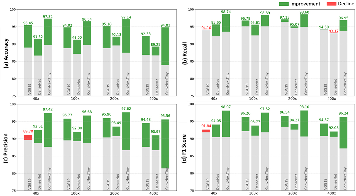
Figure 5. Performance comparison ((a) accuracy, (b) recall, (c) precision, and (d) f1 score) of the proposed method across different magnifications of the BreakHis dataset using the VGG19, DenseNet, and ConvNextTiny networks. The gray portions of the bars denote the baseline values. The green and red parts signify improvements and declines, respectively, in comparison to the baseline.
Moreover, to address the class imbalance in the BreakHis dataset, we employed the Synthetic Minority Oversampling Technique (SMOTE) [ 30 ] into the training pipeline of the ConvNextTiny network. SMOTE generates synthetic samples by interpolating between existing minority class instances, thereby enhancing their representation. This integration helps the ConvNextTiny network mitigate bias towards the majority class, enhancing its performance and robustness. Applying SMOTE improves performance and leads to identical values for accuracy, precision, recall, and F1 score as presented in Table 6. It results in more balanced predictions across both classes.
| ConvNextTiny | Magnification | Image-wise | |||||||
|---|---|---|---|---|---|---|---|---|---|
| Proposed | Baseline | ||||||||
| Accuracy | Precision | Recall | F1-score | Accuracy | Precision | Recall | F1-score | ||
| 40× | 99.14±0.44 | 99.15±0.44 | 99.14±0.44 | 99.14±0.44 | 96.32±0.54 | 96.33±0.54 | 96.32±0.54 | 96.32±0.54 | |
| 100× | 98.64±0.49 | 98.65±0.49 | 98.64±0.49 | 98.64±0.49 | 95.09±0.56 | 95.18±0.55 | 95.09±0.56 | 95.09±0.56 | |
| 200× | 98.92±0.35 | 98.92±0.35 | 98.92±0.35 | 98.92±0.35 | 95.07±0.82 | 95.10±0.81 | 95.08±0.82 | 95.07±0.82 | |
| 400× | 97.93±0.46 | 97.95±0.46 | 97.93±0.45 | 97.93±0.47 | 93.18±0.14 | 93.36±0.13 | 93.18±0.14 | 93.19±0.14 | |
In addition, the patient-wise evaluation of the proposed method on the BreakHis dataset shows also an improvement (Table 5). However, challenges arise in some cases due to the small number of images, especially in the benign category, which is the minority class (as mentioned in Table 1). In some patients, the accuracy is less than 70% at specific magnifications. The class imbalance in the dataset often leads to decisions favoring the class with more samples. In the malignant category, the proposed method results in approximately 60% accuracy for five patients at one magnification, with four of these patients belonging to a specific class (ductal carcinoma). Table 7 presents the patient-wise classification accuracy results, using the proposed method by the ConvNextTiny network, along with the number of images and tumor type for patients whose accuracies are less than 70% at least for one magnification.
| Patient’s ID | Tumor type (B: benign, M: malignant) | Accuracy/ number of images | Magnification | |||
|---|---|---|---|---|---|---|
| 40× | 100× | 200× | 400× | |||
| 16184 | Tubular adenoma (B) | Accuracy | 74.35 | 94.11 | 82.85 | 54.16 |
| Number of images | 39 | 34 | 35 | 24 | ||
| 19854C | Tubular adenoma (B) | Accuracy | 75.00 | 93.75 | 87.50 | 25.00 |
| Number of images | 16 | 16 | 16 | 16 | ||
| 21998AB | Phyllodes tumor (B) | Accuracy | 87.50 | 70.83 | 100 | 50.84 |
| Number of images | 58 | 66 | 52 | 59 | ||
| 22549CD | Adenosis (B) | Accuracy | 68.57 | 61.11 | 48.38 | 70.00 |
| Number of images | 35 | 36 | 31 | 30 | ||
| 22549G | Adenosis (B) | Accuracy | 22.85 | 52.94 | 28.12 | 41.37 |
| Number of images | 35 | 34 | 32 | 29 | ||
| 23060CD | Fibroadenoma (B) | Accuracy | 100 | 100 | 100 | 56.25 |
| Number of images | 14 | 11 | 16 | 16 | ||
| 29315EF | Phyllodes tumor (B) | Accuracy | 100 | 62.50 | 50.00 | 52.94 |
| Number of images | 13 | 16 | 14 | 17 | ||
| 190EF | Papillary carcinoma (M) | Accuracy | 78.94 | 100 | 100 | 66.66 |
| Number of images | 19 | 16 | 15 | 15 | ||
| 12312 | Ductal carcinoma (M) | Accuracy | 65.62 | 72.54 | 88.57 | 86.84 |
| Number of images | 32 | 41 | 35 | 38 | ||
| 15572 | Ductal carcinoma (M) | Accuracy | 60.86 | 100 | 100 | 86.66 |
| Number of images | 23 | 23 | 19 | 15 | ||
| 11951 | Ductal carcinoma (M) | Accuracy | 100 | 100 | 64.28 | 75.00 |
| Number of images | 27 | 25 | 28 | 20 | ||
| 15696 | Ductal carcinoma (M) | Accuracy | 100 | 91.30 | 54.54 | 100 |
| Number of images | 23 | 23 | 22 | 15 | ||
Discussion
The proposed method in this study, which involves layer selection for extracting distinctive deep features from histopathology images using MI, offers several advantages over previous ones. It is generalizable to different networks and datasets because layer selection is not done based on trial-and-error [ 8 ] or the network’s layer sequence [ 9 ]. Instead, layers are selected based on the corresponding MI values, which ensures a more informed and efficient selection process. The proposed method has also been applied to multiple networks (as shown in Figure 3) and a multi-class dataset (Figure 1b), and improved classification performance has been observed, indicating the method’s adaptability and effectiveness across different datasets and network architectures. Additionally, compared to the study that uses MI for layer selection [ 10 ], the proposed method has the advantage of not requiring classification on features extracted from each layer. This occurs because the MI is computed between features of each layer and the true labels, rather than between the model’s predicted outputs and the true labels. As a result, there is no need to perform classification with the feature vector of each layer, significantly reducing computational load and increasing processing speed. Unlike attention-based methods [ 11 , 12 ], which rely on architectural modifications and additional trainable modules, the proposed framework enhances performance through MI-based layer selection, offering a simpler and computationally efficient solution.
The selected layers from each network, as shown in Tables 2, 3, and 4, demonstrate that extracting features solely from the highest layer of the network cannot capture all the useful and distinctive features needed for image classification, and intermediate layers instead play a crucial role. While deep networks are often designed to rely heavily on the last layers to extract features, our results suggest that intermediate layers are able to provide distinctive features, particularly for histopathology image classification. For instance, in the VGG19 network, although the final layers (such as FC6 or FC7) provided improved accuracy at different magnifications [ 8 , 22 ] the intermediate layers (e.g., B5C1 and B4C2) prove to be equally, if not more, effective in capturing crucial features at same magnifications. Similarly, in DenseNet, certain middle layers (e.g., D4C5B32_1 and D3C4B30_2) play a more significant role in extracting discriminative features than the final layer. This suggests that DenseNet’s design, with its dense connectivity, may benefit more from intermediate layers rather than focusing only on the last one. In the ConvNextTiny network, layers S2B7C and S2B6C provide notable improvements in classification performance. These findings highlight the importance of layer selection in network architectures, particularly for histopathology image analysis. Furthermore, incorporating the maximum value of MI has successfully identified the effective layers in each network avoiding the common bias toward last-layer features.
From the chart shown in Figure 5, VGG19 shows improved accuracy at 40× magnification, while the other three metrics precision, F1 score, and recall do not increase compared to the baseline. Fewer details at this magnification and the imbalance dataset (as shown in Figure 1), likely contributed to this issue. DenseNet encounters difficulties at higher magnifications; as the magnification level increases and the image details become more refined, the performance improvement of the proposed method diminishes. Its architecture, where each layer receives input from all previous layers, generates similar features across layers. This redundancy, combined with the large number of parameters, leads to overfitting when the data is limited, resulting in lower overall performance. In contrast, ConvNextTiny consistently outperforms the other networks, demonstrating its ability to effectively capture complex patterns in histopathology and tissue images, even without addressing class imbalance. The design of ConvNextTiny network, inspired by ViT and its inclusion of convolutional and normalization layers, is particularly effective in capturing the complex patterns in histopathology and tissue images.
For the ICIAR/BACH dataset, the overall classification accuracy is lower due to the presence of four distinct classes and the limited number of samples, which makes it challenging to adequately learn minor differences between classes. Additionally, the limitation of implementing PCA leads to lower performance in some layers compared to the original state (before dimensionality reduction), as important information may have been lost during the reduction. However, the proposed method effectively compensates for this loss of information by combining significant and distinctive features from the selected layers, ensuring that critical information is retained to enhance classification performance.
The patient-wise evaluation of the proposed method on the BreakHis dataset also shows an improvement (Table 5). However, challenges arise in some cases due to the small number of images (Table 7), especially in the benign category, which is the minority class (as mentioned in Table 1). In some patients, the accuracy is less than 70% at specific magnifications. The class imbalance in the dataset often leads to decisions favoring the class with more samples. In the malignant category, the proposed method results in approximately 60% accuracy for five patients at one magnification, with four of these patients belonging to a specific class (ductal carcinoma).
Paired statistical tests with prior studies were not feasible due to the lack of source codes, exact model parameters, and details of data partitioning strategies. Previous works report only final performance, preventing valid statistical comparison.
Conclusion
This study proposes a MI-based method to identify the most effective layers for feature extraction in pre-trained networks and improve BC histopathology images classification. We utilized three different networks as feature extractors VGG19, DenseNet, and ConvNextTiny. Features were extracted from different layers, and the most informative layers were selected based on the maximum MI between extracted features and true labels, rather than predicted labels. This strategy substantially reduces computational cost compared with methods requiring classifier training or evaluation for every layer. After selecting the most effective layers, dimensionality reduction is applied to address feature redundancy and the imbalance between data and feature dimensions. The transformed features are then concatenated to preserve complementary information from different layers while reducing potential information loss. The proposed method improved ConvNextTiny performance by 9.25% over the baseline and achieved 82.12% accuracy. The results also show that features from the last convolutional layer do not necessarily yield the best performance, which aligns with previous studies. For the BreakHis dataset, performance varied across networks. VGG19 improved accuracy at 40× magnification but was limited by class imbalance and fewer details at this level. DenseNet struggles at higher magnifications due to feature redundancy and overfitting. However, ConvNextTiny consistently achieved better performance by effectively capturing intricate histopathology patterns. Notably, the most significant performance improvement was observed in the ConvNextTiny network, where image-wise accuracy increased by 10.88% at 400× magnification.
Despite these promising results, an important limitation remains. The feature selection process may still be impacted by redundancy or irrelevant features in complex, high-dimensional data. Future studies could introduce a more refined criterion for selecting distinguishing features from different layers that maximize MI while minimizing redundancy among selected features, leading to more compact and efficient models. Furthermore, combining advanced techniques such as attention mechanisms, which focus on the most relevant regions of the input, could enhance feature selection, potentially improving model performance in challenging datasets.
Authors’ Contribution
M. Madani and H. Shabani wrote the main manuscript and reviewed it. M. Madani contributed to software, formal analysis, visualization, and investigation. H. Shabani contributed to methodology, conceptualization, formal analysis, investigation, visualization, project administration, and supervision. All the authors read, modified, and approved the final version of the manuscript.
Ethical Approval
This study used publicly available datasets and did not involve any human or animal experiments. Therefore, ethical approval was not required.
Funding
The authors declare that no funds, grants, or other support were received during the preparation of this manuscript.
Conflict of Interest
None
Data and Code Availability Statement
The BreakHis and ICIAR datasets, which were included in the published articles [ 18 ] and [ 19 ], can be accessed at https://web.inf.ufpr.br/vri/databases/breast-cancer-histopathological-database-breakhis/ and https://iciar2018-challenge.grand-challenge.org/Dataset/, respectively. The code is available at https://github.com/labCOI/layerwise_deepfeature. The corresponding author is responsible for the implementation of the code.
References
- Rakha EA, Allison KH, Ellis IO, Horii R, Masuda S, Penault-Llorca F. WHO classification of tumours of the breast. Lyon: International Agency for Research on Cancer; 2019.
- Sung H, Ferlay J, Siegel RL, Laversanne M, Soerjomataram I, Jemal A, Bray F. Global Cancer Statistics 2020: GLOBOCAN Estimates of Incidence and Mortality Worldwide for 36 Cancers in 185 Countries. CA Cancer J Clin. 2021; 71(3):209-49. DOI | PubMed
- Boyle P, Levin B. World cancer report 2008. Lyon: International Agency for Research on Cancer; 2008.
- Elmore JG, Longton GM, Carney PA, Geller BM, Onega T, Tosteson AN, et al. Diagnostic concordance among pathologists interpreting breast biopsy specimens. JAMA. 2015; 313(11):1122-32. Publisher Full Text | DOI | PubMed [ PMC Free Article ]
- Spanhol FA, Oliveira LS, Petitjean C, Heutte L. Breast cancer histopathological image classification using convolutional neural networks. In International Joint Conference on Neural Networks (IJCNN); Vancouver, BC, Canada: IEEE; 2016.
- Stenkvist B, Westman-Naeser S, Holmquist J, Nordin B, Bengtsson E, Vegelius J, et al. Computerized nuclear morphometry as an objective method for characterizing human cancer cell populations. Cancer Res. 1978; 38(12):4688-97. PubMed
- Kashyap A, Jain M, Shukla S, Andley M. Role of Nuclear Morphometry in Breast Cancer and its Correlation with Cytomorphological Grading of Breast Cancer: A Study of 64 Cases. J Cytol. 2018; 35(1):41-5. Publisher Full Text | DOI | PubMed [ PMC Free Article ]
- Spanhol FA, Oliveira LS, Cavalin PR, Petitjean C, Heutte L. Deep features for breast cancer histopathological image classification. EEE International Conference on Systems, Man, and Cybernetics (SMC); Banff, AB, Canada: IEEE; 2017.
- Gupta V, Bhavsar A. Sequential modeling of deep features for breast cancer histopathological image classification. In Proceedings of the IEEE Conference on Computer Vision and Pattern Recognition Workshops; 2018. p. 2254-61.
- Gupta V, Bhavsar A. Partially-independent framework for breast cancer histopathological image classification. In Proceedings of the IEEE/CVF Conference on Computer Vision and Pattern Recognition Workshops; 2019.
- Zou Y, Zhang J, Huang S, Liu B. Breast cancer histopathological image classification using attention high‐order deep network. Int J Imaging Syst Technol. 2022; 32(1):266-79. DOI
- Ashurov A, Chelloug SA, Tselykh A, Muthanna MSA, Muthanna A, Al-Gaashani MSAM. Improved Breast Cancer Classification through Combining Transfer Learning and Attention Mechanism. Life (Basel). 2023; 13(9):1945. Publisher Full Text | DOI | PubMed [ PMC Free Article ]
- Roy S, Jain PK, Tadepalli K, Reddy BP. Forward attention-based deep network for classification of breast histopathology image. Multimed Tools Appl. 2024; 83(40):88039-68. DOI
- Lakshmi Priya CV, Biju VG, Vinod BR, Ramachandran S. Deep learning approaches for breast cancer detection in histopathology images: A review. Cancer Biomark. 2024; 40(1):1-25. Publisher Full Text | DOI | PubMed [ PMC Free Article ]
- Al-Antari MA, Al-Masni MA, Choi MT, Han SM, Kim TS. A fully integrated computer-aided diagnosis system for digital X-ray mammograms via deep learning detection, segmentation, and classification. Int J Med Inform. 2018; 117:44-54. DOI | PubMed
- Pan SJ, Yang Q. A survey on transfer learning. IEEE Trans Knowl Data Eng. 2009; 22(10):1345-59. DOI
- Azmoodeh-Kalati M, Shabani H, Maghareh MS, Barzegar Z, Lashgari R. Leveraging an ensemble of EfficientNetV1 and EfficientNetV2 models for classification and interpretation of breast cancer histopathology images. Sci Rep. 2025; 15(1):21541. Publisher Full Text | DOI | PubMed [ PMC Free Article ]
- Spanhol FA, Oliveira LS, Petitjean C, Heutte L. A Dataset for Breast Cancer Histopathological Image Classification. IEEE Trans Biomed Eng. 2016; 63(7):1455-62. DOI | PubMed
- Araújo T, Aresta G, Castro E, Rouco J, Aguiar P, Eloy C, et al. Classification of breast cancer histology images using Convolutional Neural Networks. PLoS One. 2017; 12(6):e0177544. Publisher Full Text | DOI | PubMed [ PMC Free Article ]
- Zeiler MD, Fergus R. Visualizing and understanding convolutional networks. In European conference on computer vision Cham: Springer; 2014.
- He K, Zhang X, Ren S, Sun J. Deep residual learning for image recognition. In IEEE Conference on Computer Vision and Pattern Recognition (CVPR): IEEE; 2016.
- Morovati B, Lashgari R, Hajihasani M, Shabani H. Reduced Deep Convolutional Activation Features (R-DeCAF) in Histopathology Images to Improve the Classification Performance for Breast Cancer Diagnosis. J Digit Imaging. 2023; 36(6):2602-12. Publisher Full Text | DOI | PubMed [ PMC Free Article ]
- Zisserman A. Very deep convolutional networks for large-scale image recognition [Internet]. arXiv [Preprint]. 2014 [cited 2014 Sep 4]. Available from: https://arxiv.org/abs/1409.1556
- Huang G, Liu Z, Van Der Maaten L, Weinberger KQ. Densely connected convolutional networks. InProceedings of the IEEE conference on computer vision and pattern recognition; CVPR; 2017. p. 4700-8.
- Liu Z, Mao H, Wu CY, Feichtenhofer C, Darrell T, Xie S. A convnet for the 2020s. In Proceedings of the IEEE/CVF Conference on Computer Vision and Pattern Recognition; 2022. p. 11976-86.
- Ross BC. Mutual information between discrete and continuous data sets. PLoS One. 2014; 9(2):e87357. Publisher Full Text | DOI | PubMed [ PMC Free Article ]
- Subramanian J, Simon R. Overfitting in prediction models - is it a problem only in high dimensions? Contemp Clin Trials. 2013; 36(2):636-41. DOI | PubMed
- Murphy KP. Machine learning: A probabilistic perspective. Cambridge, MA: MIT Press; 2012.
- Kumar A, Singh SK, Saxena S, Lakshmanan K, Sangaiah AK, Chauhan H, et al. Deep feature learning for histopathological image classification of canine mammary tumors and human breast cancer. Inf Sci. 2020; 508:405-21. DOI
- Chawla NV, Bowyer KW, Hall LO, Kegelmeyer WP. SMOTE: synthetic minority over-sampling technique. J Artif Intell Res. 2002; 16:321-57. DOI


